roi-based MVPA with group-analysis
Load t-stat data from all subjects, apply 'vt' mask, compute difference of (fisher-transformed) between on- and off diagonal split-half correlation values, and perform a random effects analysis.
- For CoSMoMVPA's copyright information and license terms, #
- see the COPYING file distributed with CoSMoMVPA. #
Contents
Set analysis parameters
subject_ids = {'s01', 's02', 's03', 's04', 's05', 's06', 's07', 's08'};
rois = {'ev'; 'vt'; 'brain'};
labels = {'monkey'; 'lemur'; 'mallard'; 'warbler'; 'ladybug'; 'lunamoth'};

nsubjects = numel(subject_ids);

% allocate space for output
sum_weighted_zs_all = zeros(nsubjects, 1);

config = cosmo_config();
study_path = fullfile(config.tutorial_data_path, 'ak6');
Loop over rois
nrois = numel(rois);
for i_roi = 1:nrois
    % pre-allocate space weighted correlation difference
    % in each subject
    sum_weighted_zs_all = zeros(nsubjects, 1);
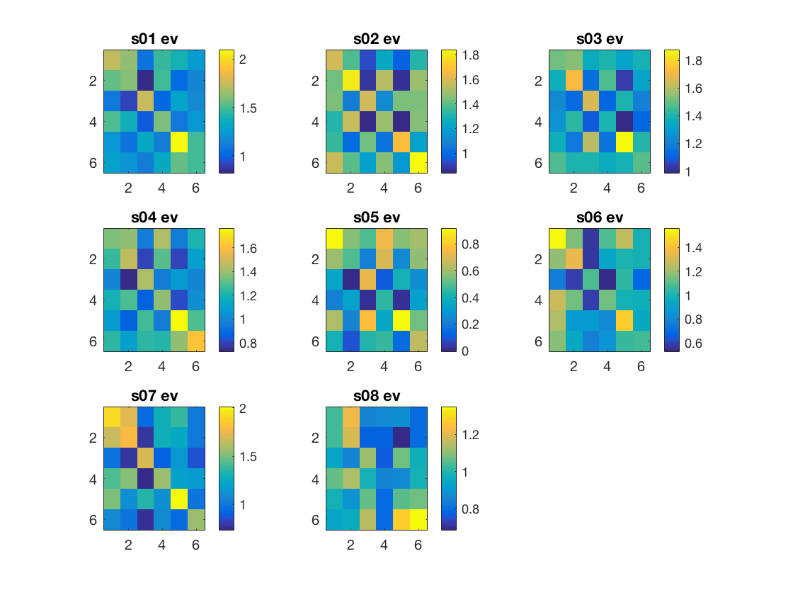
Computations for each subject
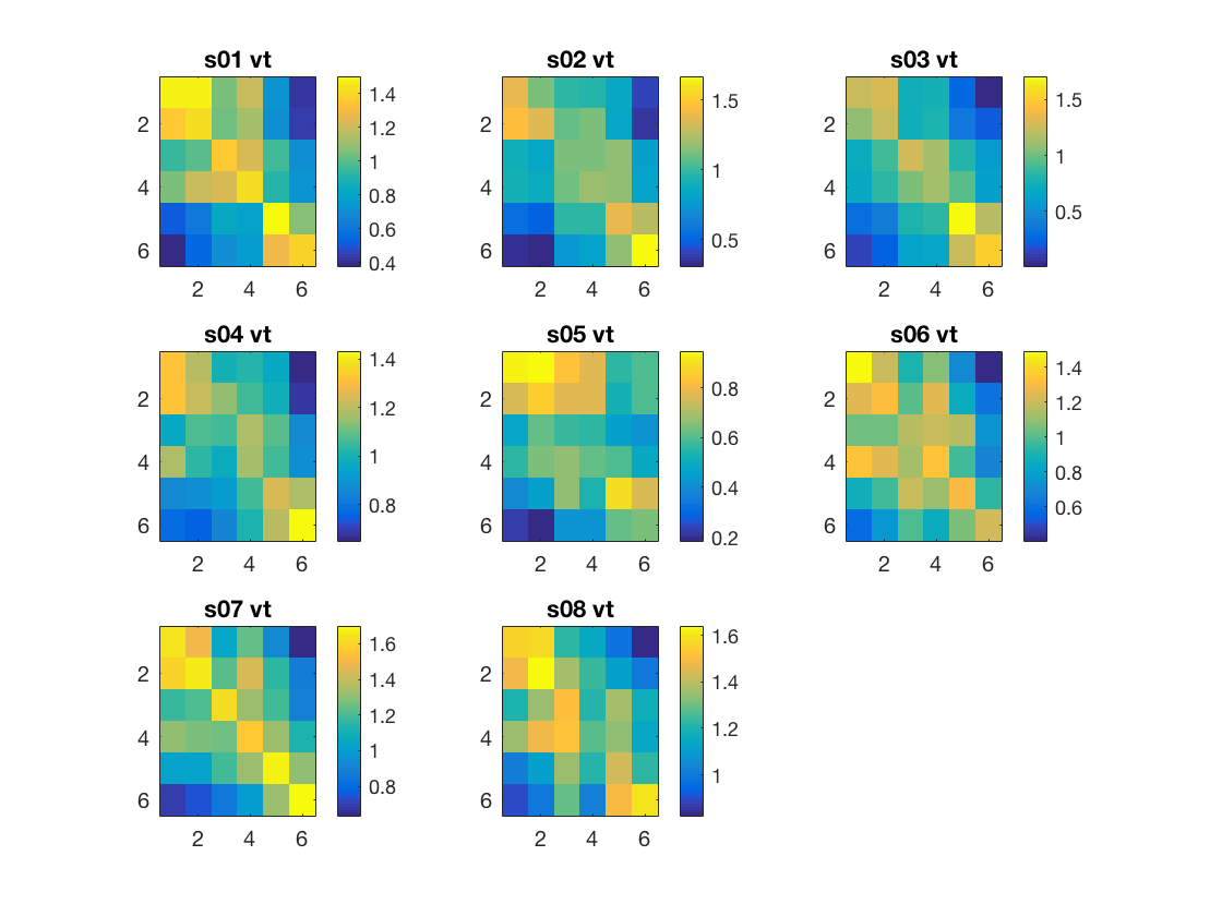
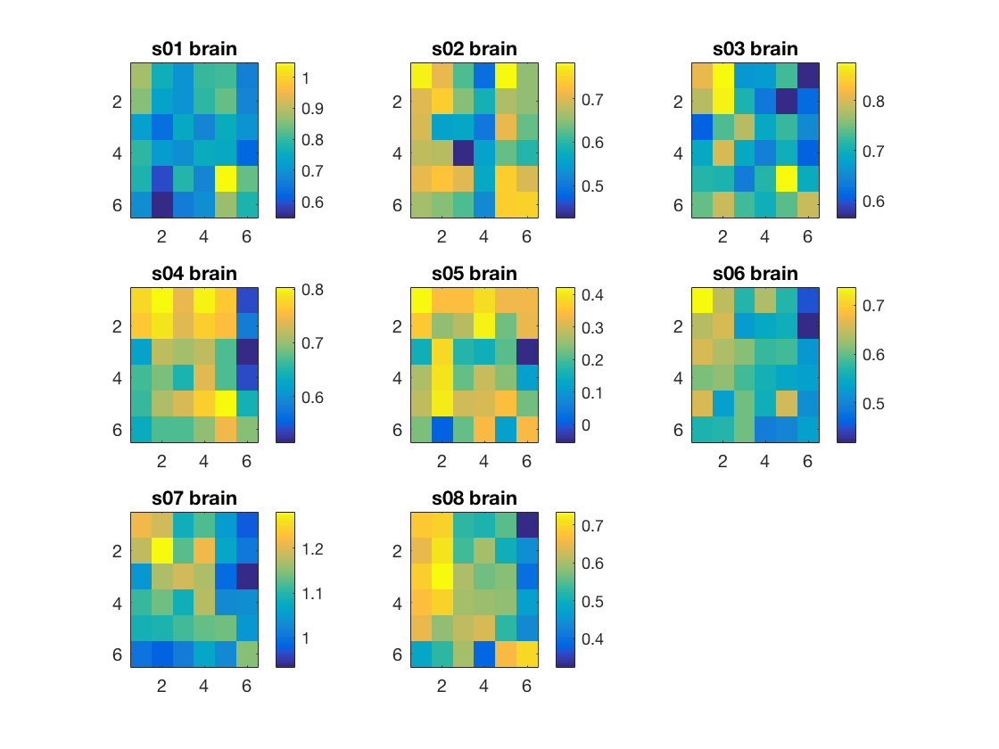
    for i_subj = 1:nsubjects
        subject_id = subject_ids{i_subj};

        data_path = fullfile(study_path, subject_id);

        % file locations for both halves
        half1_fn = fullfile(data_path, 'glm_T_stats_odd.nii');
        half2_fn = fullfile(data_path, 'glm_T_stats_even.nii');

        % mask name for given subject and roi
        mask_fn = fullfile(data_path, [rois{i_roi}, '_mask.nii']);

        % load two halves as CoSMoMVPA dataset structs.
        half1_ds = cosmo_fmri_dataset(half1_fn, 'mask', mask_fn);
        half2_ds = cosmo_fmri_dataset(half2_fn, 'mask', mask_fn);

        % get the sample data
        % each half has six samples:
        % monkey, lemur, mallard, warbler, ladybug, lunamoth.
        half1_samples = half1_ds.samples;
        half2_samples = half2_ds.samples;

        % compute all correlation values between the two halves, resulting
        % in a 6x6 matrix. Store this matrix in a variable 'rho'.
        % Hint: use cosmo_corr
        % >@@>
        rho = cosmo_corr(half1_samples', half2_samples');
        % <@@<

        % for the advanced exercise ('compute the average of all individual
        % correlation matrices'): if the first subject and roi,
        % allocate space for a 'rho_sum' array with three dimensions;
        % the first two dimensions for the two halves, the third
        % one for different rois.
        % Then add 'rho' to 'rho_sum'
        %
        % (If you don't want to do the advanced
        % exercise, yo don't have to do anything here.)
        % >@@>
        if i_subj == 1 && i_roi == 1
            % first correlation was just computed, and we now know
            % the number of conditions through the size of rho.
            %
            % allocate space for sum over subjects
            nclasses = size(rho, 1);
            rho_sum = zeros([nclasses, nclasses, nrois]);
        end
        rho_sum(:, :, i_roi) = rho_sum(:, :, i_roi) + rho;

        % <@@<

        % To make these correlations more 'normal', apply a Fisher
        % transformation and store this in a variable 'z' (use atanh).
        % >@@>
        z = atanh(rho);
        % <@@<

        % visualize the matrix 'z'
        subplot(3, 3, i_subj);
        % >@@>
        imagesc(z);
        colorbar();
        title([subject_id ' ' rois{i_roi}]);
        % <@@<

        % define in a variable 'contrast_matrix' how correlations values
        % are going to be weighted.
        % The matrix must have a mean of zero, positive values on diagonal,
        % negative elsewhere.

        nclasses = size(rho, 1);
        % sanity check; in this example there are 6 conditions
        assert(nclasses == 6);

        % set contrast matrix. It has a mean of zero, the diagonal elements
        % sum to 1, and the non-diagonal element sum to -1
        contrast_matrix = (eye(nclasses) - 1 / nclasses) / (nclasses - 1);

        if abs(mean(contrast_matrix(:))) > 1e-14
            error('illegal contrast matrix');
        end

        % Weigh the values in the matrix 'z' by those in the
        % contrast_matrix and then sum them (hint: use the '.*'
        % operator for element-wise multiplication). Store the results in
        % a variable 'sum_weighted_z'.
        % >@@>
        weighted_z = z .* contrast_matrix;

        sum_weighted_z = sum(weighted_z(:));
        % <@@<

        % store the result for this subject in sum_weighted_zs_all
        % (at the i_subj-th position), so that
        % group statistics can be computed
        % >@@>
        sum_weighted_zs_all(i_subj) = sum_weighted_z;
        % <@@<
    end
compute t statistic and print the result
run one-sample t-test again zero
    % Using matlab's stat toolbox (if present)
    if cosmo_check_external('@stats', false)

        % >@@>
        [h, p, ci, stats] = ttest(sum_weighted_zs_all);
        fprintf(['correlation difference in %s at group level: '...
                 '%.3f +/- %.3f, t_%d=%.3f, p=%.5f (using matlab stats '...
                 'toolbox)\n'], ...
                rois{i_roi}, mean(sum_weighted_zs_all), ...
                std(sum_weighted_zs_all), ...
                stats.df, stats.tstat, p);
        % <@@<
    else
        fprintf('Matlab stats toolbox not available\n');
    end

    % Apart from using the 'ttest' function (if available), one can
    % also use 'cosmo_stat' for univaraite statistics.
    % For this approach, data must be represented in a dataset struct.
    %
    % The targets are chunks are set to indicate that all samples are from
    % the same class (condition), and each observation is independent from
    % the others
    sum_weighted_zs_ds = struct();
    sum_weighted_zs_ds.samples = sum_weighted_zs_all;
    sum_weighted_zs_ds.sa.targets = ones(nsubjects, 1);
    sum_weighted_zs_ds.sa.chunks = (1:nsubjects)';

    ds_t = cosmo_stat(sum_weighted_zs_ds, 't');     % t-test against zero
    ds_p = cosmo_stat(sum_weighted_zs_ds, 't', 'p'); % convert to p-value

    fprintf(['correlation difference in %s at group level: '...
             '%.3f +/- %.3f, %s=%.3f, p=%.5f (using cosmo_stat)\n'], ...
            rois{i_roi}, mean(sum_weighted_zs_all), std(sum_weighted_zs_all), ...
            ds_t.sa.stats{1}, ds_t.samples, ds_p.samples);
correlation difference in ev at group level: 0.379 +/- 0.137, t_7=7.854, p=0.00010 (using matlab stats toolbox)
correlation difference in ev at group level: 0.379 +/- 0.137, Ttest(7)=7.854, p=0.00010 (using cosmo_stat)
correlation difference in vt at group level: 0.397 +/- 0.163, t_7=6.864, p=0.00024 (using matlab stats toolbox)
correlation difference in vt at group level: 0.397 +/- 0.163, Ttest(7)=6.864, p=0.00024 (using cosmo_stat)
correlation difference in brain at group level: 0.074 +/- 0.026, t_7=7.987, p=0.00009 (using matlab stats toolbox)
correlation difference in brain at group level: 0.074 +/- 0.026, Ttest(7)=7.987, p=0.00009 (using cosmo_stat)
end
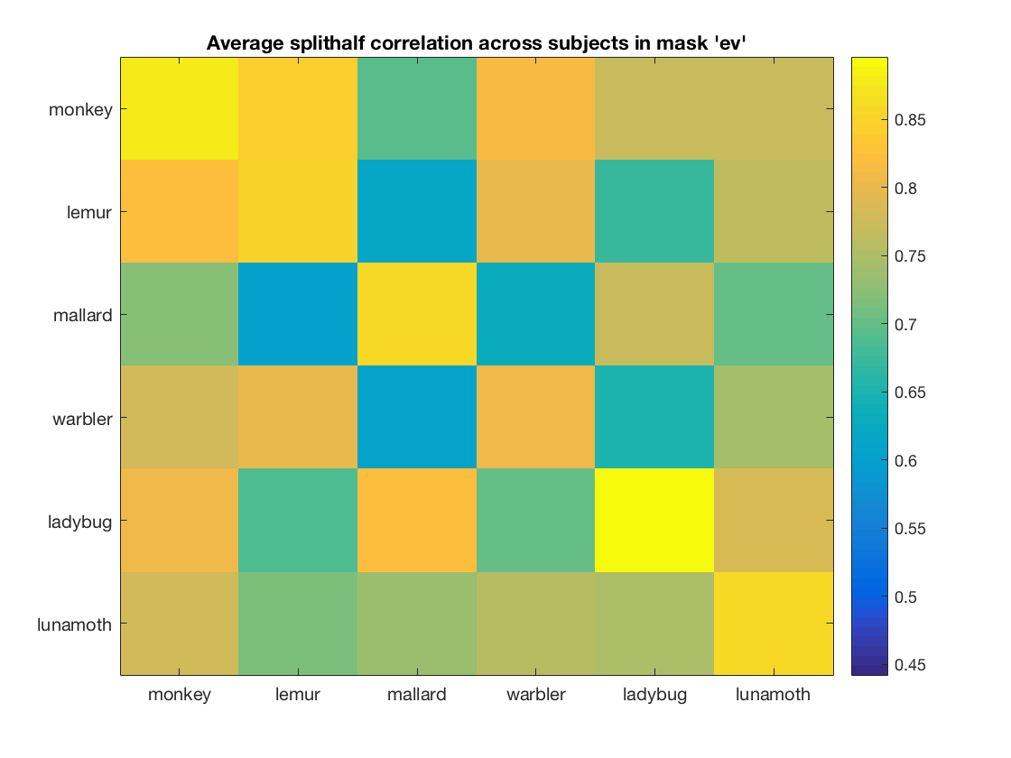
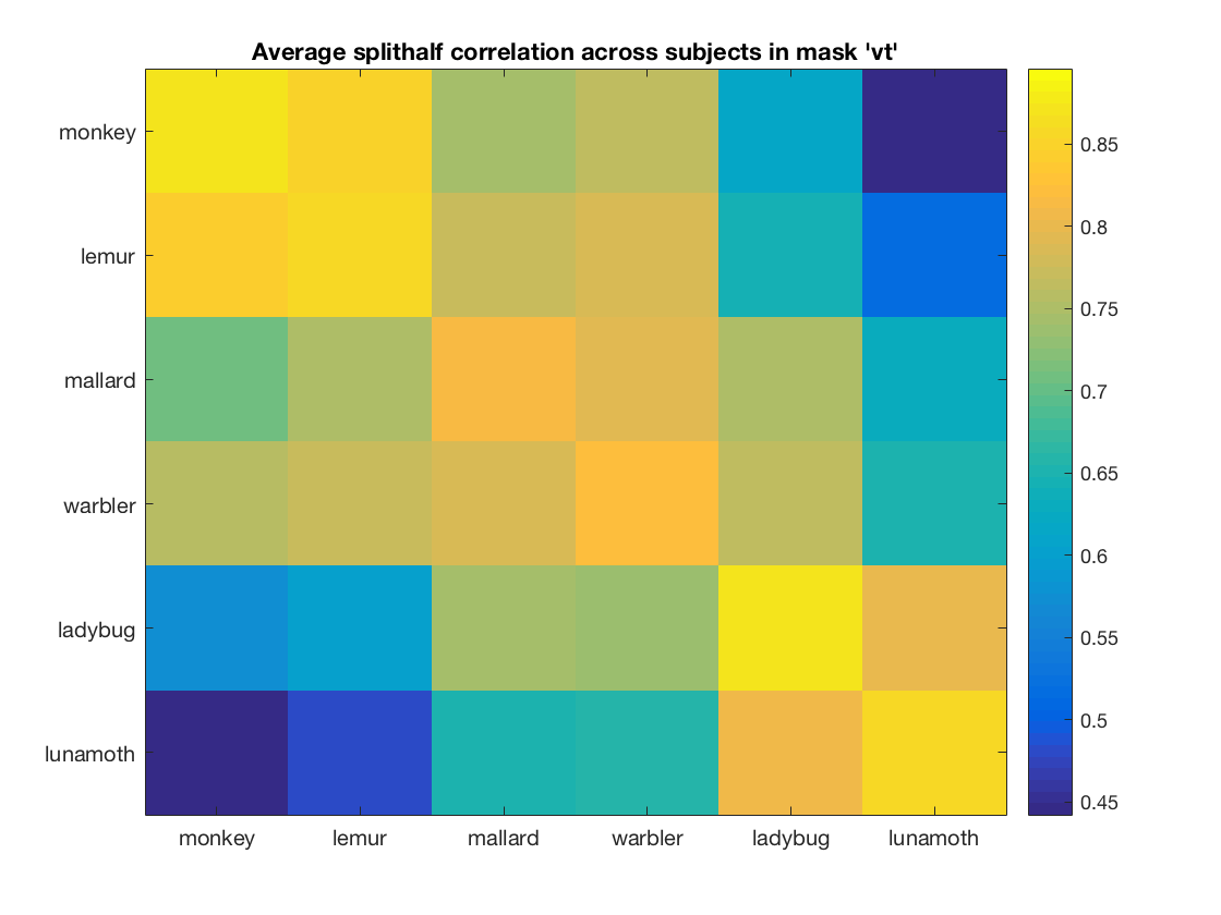
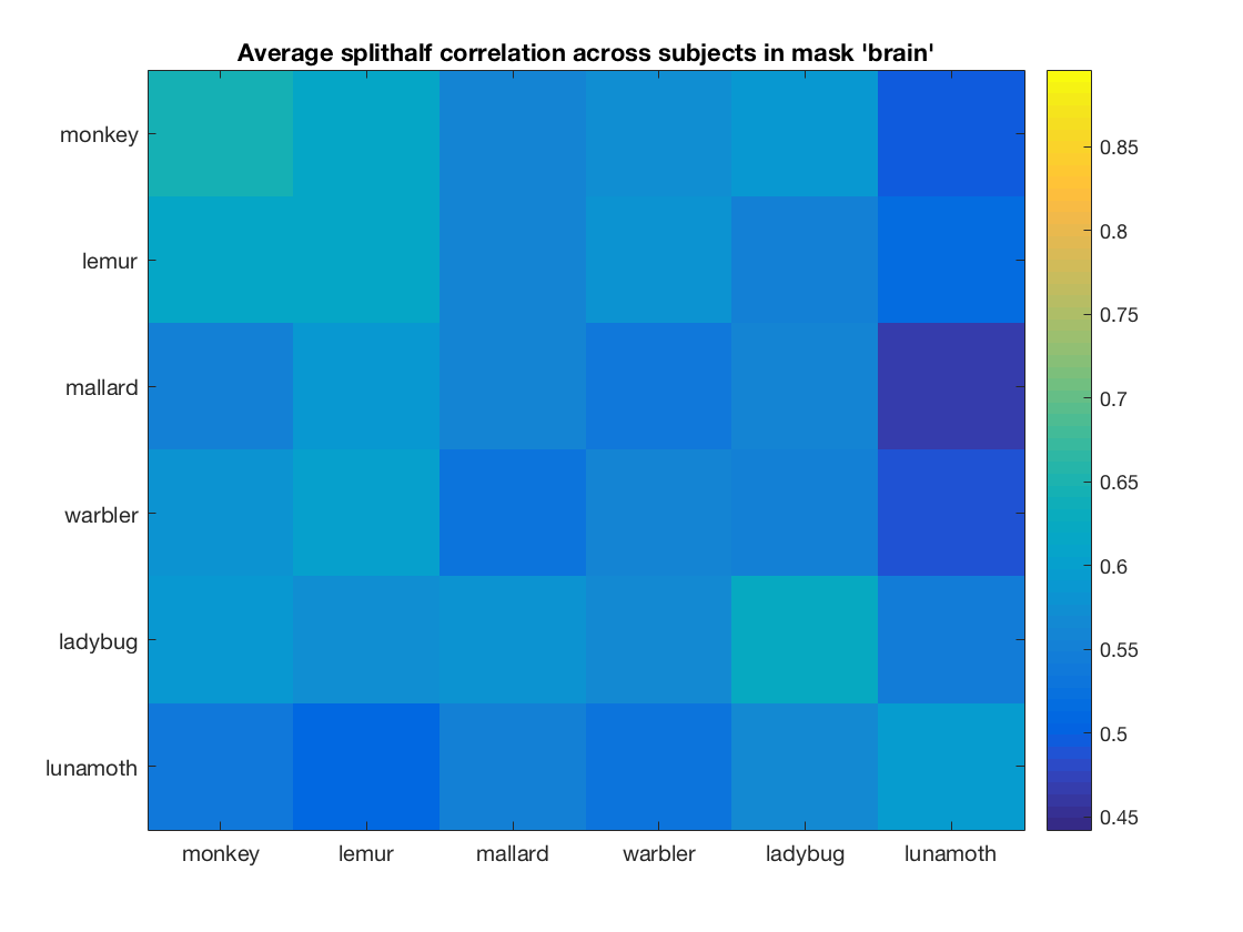
advanced exercise
% plot an image of the correlation matrix averaged over
% participants (one for each roi)

% allocate space for axis handles, so that later all plots can be set to
% have the same color limits
ax_handles = zeros(nrois, 1);
col_limits = zeros(nrois, 2);

for i_roi = 1:nrois
    figure;

    % store axis handle for current figure
    ax_handles(i_roi) = gca;

    % compute the average correlation matrix using 'rho_sum', and store the
    % result in a variable 'rho_mean'. Note that the number of subjects is
    % stored in a variable 'nsubjects'
    % >@@>
    rho_mean = rho_sum(:, :, i_roi) / nsubjects;
    % <@@<

    % visualize the rho_mean matrix using imagesc
    % >@@>
    imagesc(rho_mean);
    % <@@<

    % set labels, colorbar and title
    set(gca, 'xtick', 1:numel(labels), 'xticklabel', labels);
    set(gca, 'ytick', 1:numel(labels), 'yticklabel', labels);

    colorbar;
    desc = sprintf(['Average splithalf correlation across subjects '...
                    'in mask ''%s'''], rois{i_roi});
    title(desc);

    col_limits(i_roi, :) = get(gca, 'clim');
end

% give all figures the same color limits such that correlations can be
% compared visually
set(ax_handles, 'clim', [min(col_limits(:)), max(col_limits(:))]);