MEEG time-lock searchlight
This example shows MVPA analyses performed on MEEG data.
The input dataset involved a paradigm with electrical median nerve stimulation for durations of 2s at 20Hz.
Using a time-channel neighborhood, a searchlight map is computed indicating in time and space (channel) the pre-stimulation period can be distinguished from the peri/post stimulation period.
The code presented here can be adapted for other MEEG analyses, but there are a few potential caveats: * assignment of targets (labels of conditions) is based here on stimulation periods versus pre-stimulation periods. In typical analyses the targets should be based on different trial conditions, for example as set a FieldTrip .trialinfo field. * assignment of chunks (parts of the data that are assumed to be independent) is based on a trial-by-trial basis. For cross-validation, the number of chunks is reduced to two to speed up the analysis. * the current examples do not perform baseline corrections or signal normalizations, which may reduce discriminatory power.
Note: running this code requires FieldTrip.
- For CoSMoMVPA's copyright information and license terms, #
- see the COPYING file distributed with CoSMoMVPA. #
Contents
get timelock data in CoSMoMVPA format
% set configuration
config=cosmo_config();
data_path=fullfile(config.tutorial_data_path,'meg_20hz');

% show dataset information
readme_fn=fullfile(data_path,'README');
cosmo_type(readme_fn);

% reset citation list
cosmo_check_external('-tic');

% load data
data_fn=fullfile(data_path,'subj102_B01_20Hz_timelock.mat');
data_tl=load(data_fn);

% convert to cosmomvpa struct
ds_tl=cosmo_meeg_dataset(data_tl);

% set the target (trial condition)
ds_tl.sa.targets=ds_tl.sa.trialinfo(:,1); % 1=pre, 2=post

% set the chunks (independent measurements)
% in this dataset, the first half of the samples (in order)
% are the post-trials;
% the second half the pre-trials
ds_tl.sa.chunks=[(1:145) (1:145)]';


% in addition give a label to each trial
index2label={'pre','post'}; % 1=pre, 2=peri/post
ds_tl.sa.labels=cellfun(@(x)index2label(x),num2cell(ds_tl.sa.targets));

% just to check everything is ok
cosmo_check_dataset(ds_tl);

% get rid of features with at least one NaN value across samples
fa_nan_mask=sum(isnan(ds_tl.samples),1)>0;
fprintf('%d / %d features have NaN\n', ...
            sum(fa_nan_mask), numel(fa_nan_mask));
ds_tl=cosmo_slice(ds_tl, ~fa_nan_mask, 2);
Summary
-------
MEG data in raw, time-locked and time-frequency formats.

Contents
--------
- subj102_B01_20Hz.fif            raw MEG recording
- preproc.m                       Matlab preprocessing script (based on
                                  FieldTrip)
- subj102_B01_20Hz_timefreq.mat   Time-locked data (generated by preproc.m)
- subj102_B01_20Hz_timelock.mat   Time-frequency data  (generated by preproc.m)
- LICENSE                         License file
- README                          This file

Methods
-------
The dataset involved a paradigm with electrical median nerve stimulation with a
human participant for durations of 2s at 20Hz. Data was acquired at 1khz using
a neuromag306 system.
Trial info in the .mat files: 1=pre-stimulus, 2=peri/post-stimulus

License
-------
The contents are made available by Nathan Weisz <nathanweisz |at| me.com> and
Gianpaolo Demarchi <gianpaolo.demarchi |at| unitn.it> under the Creative
Commons CC0 1.0 Universal Public Domain Dedication ("CC0"). See the LICENSE
file for details, or visit
http://creativecommons.org/publicdomain/zero/1.0/deed.en.

Acknowledgements
----------------
Thanks to Nathan Weisz and Gianpaolo Demarchi for providing this dataset, and
an anonymous participant for volunteering during the recordings.

Contact
-------
Nikolaas N. Oosterhof <nikolaas.oosterhof |at| unitn.it>
0 / 60600 features have NaN
set MVPA parameters
fprintf('The input has feature dimensions %s\n', ...
                cosmo_strjoin(ds_tl.a.fdim.labels,', '));


% set chunks
% again for speed just two chunks
% (targets were already set above)
nchunks=2;
ds_tl.sa.chunks=cosmo_chunkize(ds_tl, nchunks);

% define neighborhood parameters for each dimension

% channel neighborhood uses meg_combined_from_planar, which means that the
% input are planar channels but the output has combined-planar channels.
% to use the magnetometers, use 'meg_axial'
chan_type='meg_combined_from_planar';
chan_count=10;        % use 10 channel locations (relative to the combined
                      % planar channels)
                      % as we use meg_combined_from_planar there are
                      % 20 channels in each searchlight because
                      % gradiometers are paired
time_radius=2; % 2*2+1=5 time bines

% define the neighborhood for each dimensions
chan_nbrhood=cosmo_meeg_chan_neighborhood(ds_tl, 'count', chan_count, ...
                                                'chantype', chan_type);
time_nbrhood=cosmo_interval_neighborhood(ds_tl,'time',...
                                            'radius',time_radius);

% cross neighborhoods for chan-time searchlight
nbrhood=cosmo_cross_neighborhood(ds_tl,{chan_nbrhood,...
                                        time_nbrhood});

% print some info
nbrhood_nfeatures=cellfun(@numel,nbrhood.neighbors);
fprintf('Features have on average %.1f +/- %.1f neighbors\n', ...
            mean(nbrhood_nfeatures), std(nbrhood_nfeatures));

% only keep features with at least 10 neighbors
center_ids=find(nbrhood_nfeatures>10);

% for illustration purposes use the split-half measure because it is
% relatively fast - but clasifiers can also be used
measure=@cosmo_correlation_measure;

% split-half, as there are just two chunks
% (when using a classifier, do not use 'half' but the number of chunks to
% leave out for testing, e.g. 1).
measure_args=struct();
measure_args.partitions=cosmo_nchoosek_partitioner(ds_tl,'half');
The input has feature dimensions chan, time
+00:00:01 [####################] -00:00:00  crossing neighborhoods
Features have on average 98.3 +/- 4.9 neighbors
run searchlight
sl_tl_ds=cosmo_searchlight(ds_tl,nbrhood,measure,measure_args,...
                                      'center_ids',center_ids);
+00:00:18 [####################] -00:00:00
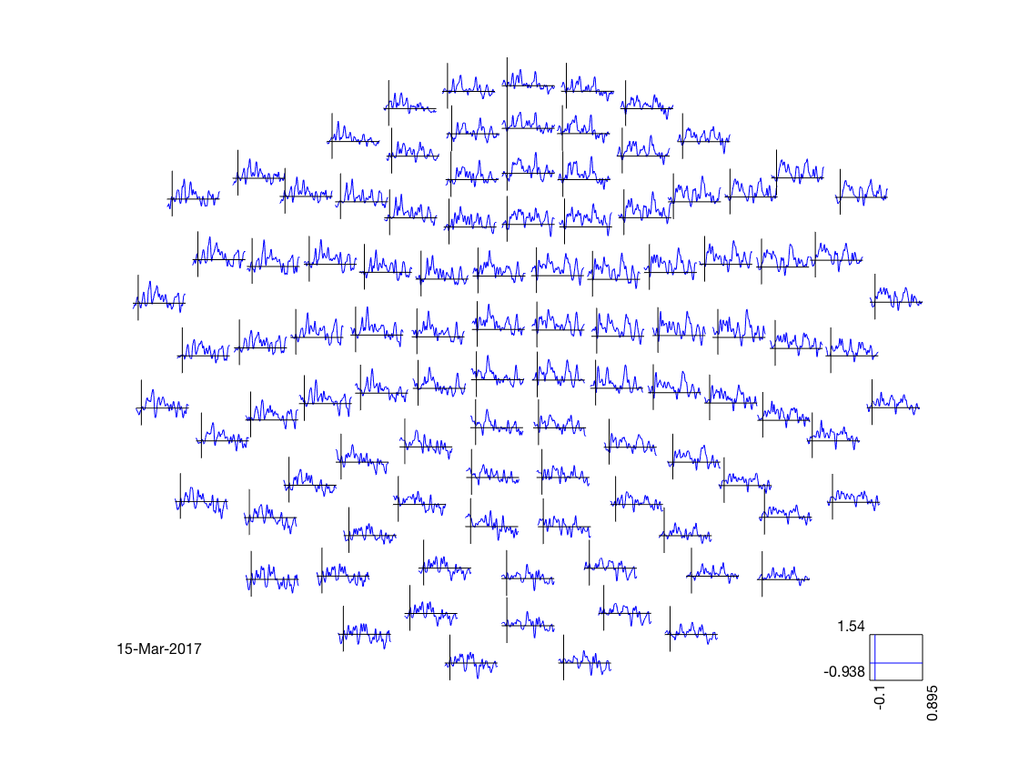
visualize timeseries results
% deduce layout from output
layout=cosmo_meeg_find_layout(sl_tl_ds);
fprintf('The output uses layout %s\n', layout.name);

% map to FT struct for visualization
sl_tl_ft=cosmo_map2meeg(sl_tl_ds);

figure();
cfg = [];
cfg.interactive = 'yes';
cfg.zlim=[-1 1];
cfg.layout       = layout;

% show figure with plots for each sensor
ft_multiplotER(cfg, sl_tl_ft);
The output uses layout neuromag306cmb.lay
the call to "ft_selectdata" took 0 seconds and required the additional allocation of an estimated 31 MB
the call to "ft_prepare_layout" took 0 seconds and required the additional allocation of an estimated 0 MB
the call to "ft_multiplotER" took 3 seconds and required the additional allocation of an estimated 53 MB
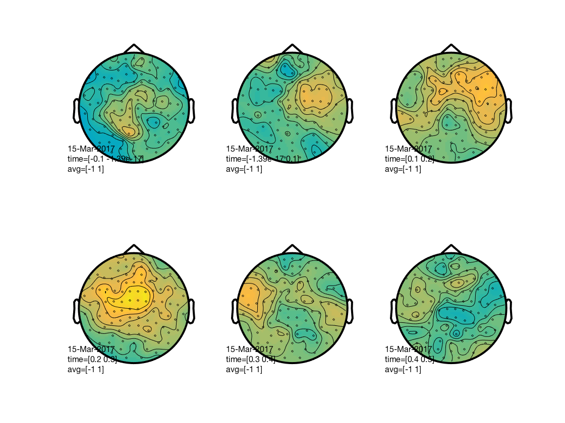
visualize topology results
show figure with topology for 0 to 600ms after stimulus onset in bins of 100 ms
figure();
cfg.xlim=-0.1:0.1:0.5;
ft_topoplotER(cfg, sl_tl_ft);
the call to "ft_prepare_layout" took 0 seconds and required the additional allocation of an estimated 0 MB
the call to "ft_prepare_layout" took 0 seconds and required the additional allocation of an estimated 0 MB
the call to "ft_topoplotTFR" took 1 seconds and required the additional allocation of an estimated 18 MB
the call to "ft_prepare_layout" took 0 seconds and required the additional allocation of an estimated 0 MB
the call to "ft_topoplotTFR" took 1 seconds and required the additional allocation of an estimated 4 MB
the call to "ft_prepare_layout" took 0 seconds and required the additional allocation of an estimated 0 MB
the call to "ft_topoplotTFR" took 1 seconds and required the additional allocation of an estimated 6 MB
the call to "ft_prepare_layout" took 0 seconds and required the additional allocation of an estimated 0 MB
the call to "ft_topoplotTFR" took 1 seconds and required the additional allocation of an estimated 5 MB
the call to "ft_prepare_layout" took 0 seconds and required the additional allocation of an estimated 0 MB
the call to "ft_topoplotTFR" took 1 seconds and required the additional allocation of an estimated 5 MB
the call to "ft_prepare_layout" took 0 seconds and required the additional allocation of an estimated 0 MB
the call to "ft_topoplotTFR" took 1 seconds and required the additional allocation of an estimated 1 MB
the call to "ft_topoplotER" took 5 seconds and required the additional allocation of an estimated 43 MB
Show citation information
cosmo_check_external('-cite');
If you use CoSMoMVPA and/or some other toolboxes for a publication, please cite:

R. Oostenveld, P. Fries, E. Maris, J.-M. Schoffelen (2011). FieldTrip: Open Source Software for Advanced Analysis of MEG, EEG, and Invasive Electrophysiological Data, Computational Intelligence and Neuroscience, vol. 2011, Article ID 156869, 9 pages.doi:10.1155/2011/156869. FieldTrip toolbox available online from http://fieldtrip.fcdonders.nl

N. N. Oosterhof, A. C. Connolly, J. V. Haxby (2016). CoSMoMVPA: multi-modal multivariate pattern analysis of neuroimaging data in Matlab / GNU Octave. Frontiers in Neuroinformatics, doi:10.3389/fninf.2016.00027.. CoSMoMVPA toolbox available online from http://cosmomvpa.org

The Mathworks, Natick, MA, United States. Matlab 9.1.0.441655 (R2016b) (September 7, 2016). available online from http://www.mathworks.com