MEEG dataset operations

This example shows MVPA analyses performed on MEEG data.

The input dataset involved a paradigm with electrical median nerve stimulation for durations of 2s at 20Hz.

The code presented here can be adapted for other MEEG analyses, but there are a few potential caveats: * assignment of targets (labels of conditions) is based here on stimulation periods versus pre-stimulation periods. In typical analyses the targets should be based on different trial conditions, for example as set a FieldTrip .trialinfo field. * assignment of chunks (parts of the data that are assumed to be independent) is done randomly. In typical analyses they can be based on different runs, with one chunk value per run. * the time window used for analyses is rather small. This means that in particular for time-freq analysis a lot of data is missing, especially for early and late timepoints in the lower frequency bands. For typical analyses it may be preferred to use a wider time window. * the current examples do not perform baseline corrections or signal normalizations, which may reduce discriminatory power.

Note: running this code requires FieldTrip.

Contents

get timelock data in CoSMoMVPA format

% set configuration
config=cosmo_config();
data_path=fullfile(config.tutorial_data_path,'meg_20hz');

% show dataset information
readme_fn=fullfile(data_path,'README');
cosmo_type(readme_fn);

% reset citation list
cosmo_check_external('-tic');

% load data
data_fn=fullfile(data_path,'subj102_B01_20Hz_timelock.mat');
data_tl=load(data_fn);

% convert to cosmomvpa struct
ds_tl=cosmo_meeg_dataset(data_tl);

% set the target (trial condition)
ds_tl.sa.targets=ds_tl.sa.trialinfo(:,1); % 1=pre, 2=post

% in addition give a label to each trial
index2label={'pre','post'}; % 1=pre, 2=peri/post
ds_tl.sa.labels=cellfun(@(x)index2label(x),num2cell(ds_tl.sa.targets));

% just to check everything is ok
cosmo_check_dataset(ds_tl);

Summary
-------
MEG data in raw, time-locked and time-frequency formats.

Contents
--------
- subj102_B01_20Hz.fif            raw MEG recording
- preproc.m                       Matlab preprocessing script (based on 
                                  FieldTrip)
- subj102_B01_20Hz_timefreq.mat   Time-locked data (generated by preproc.m)
- subj102_B01_20Hz_timelock.mat   Time-frequency data  (generated by preproc.m)
- LICENSE                         License file 
- README                          This file

Methods
-------
The dataset involved a paradigm with electrical median nerve stimulation with a 
human participant for durations of 2s at 20Hz. Data was acquired at 1khz using 
a neuromag306 system. 
Trial info in the .mat files: 1=pre-stimulus, 2=peri/post-stimulus

License
-------
The contents are made available by Nathan Weisz <nathanweisz |at| me.com> and 
Gianpaolo Demarchi <gianpaolo.demarchi |at| unitn.it> under the Creative 
Commons CC0 1.0 Universal Public Domain Dedication ("CC0"). See the LICENSE 
file for details, or visit 
http://creativecommons.org/publicdomain/zero/1.0/deed.en.

Acknowledgements
----------------
Thanks to Nathan Weisz and Gianpaolo Demarchi for providing this dataset, and 
an anonymous participant for volunteering during the recordings.

Contact
-------
Nikolaas N. Oosterhof <nikolaas.oosterhof |at| unitn.it>

Print some information about dataset

% print the size. Note that the number of features is the number of time
% points times the number of channels.
[ns,nf]=size(ds_tl.samples);
fprintf('There are %d samples and %d features\n', ns, nf);

fdim_labels=ds_tl.a.fdim.labels;
fdim_values=ds_tl.a.fdim.values;
ndim=numel(fdim_labels);
for dim=1:ndim
    dim_label=fdim_labels{dim};
    nvalues=numel(fdim_values{dim});
    fprintf('Dimension %d (%s) has %d values\n', dim, dim_label, nvalues);
end

There are 290 samples and 60600 features
Dimension 1 (chan) has 303 values
Dimension 2 (time) has 200 values

Simple data manipulations

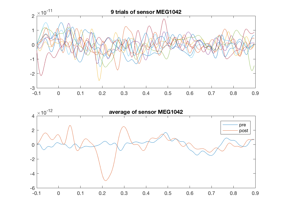
select five trials from post-stim period

post_mask=cosmo_match(ds_tl.sa.labels,'post');
ds_tl_post=cosmo_slice(ds_tl,post_mask);
select_trials=2:2:18;

% the last argument indicates to slice along the first dimension.
% The value 1 is the default and can be omitted
ds_trial=cosmo_slice(ds_tl_post, select_trials, 1);

% select a single channel (multiple channels are also possible but
% makes plotting the samples directly a bit more tricky)
chan={'MEG1042'};
chan_msk=cosmo_dim_match(ds_trial,'chan', chan);

% slice again, this time along the feature dimension (dimension 2),
% to get a new dataset with just one channel
ds_trial_chan=cosmo_slice(ds_trial, chan_msk, 2);

% plot five individual trials
figure();
subplot(2,1,1);
plot(data_tl.time, ds_trial_chan.samples');
title(sprintf('%d trials of sensor %s', numel(select_trials), chan{1}));

% use original full data to select data in just one channel
chan_msk=cosmo_dim_match(ds_tl,'chan', chan);
ds_chan=cosmo_slice(ds_tl, chan_msk, 2);

ds_mean=cosmo_fx(ds_chan,@(x)mean(x,1),'targets');
% plot signal time course averaged over all samples
% note: the 'pre' data has been shifted in time to match the 'post' data
subplot(2,1,2);
[time_dim, time_index]=cosmo_dim_find(ds_mean,'time');
assert(time_dim==2); % it is a feature dimension
plot(ds_mean.a.fdim.values{time_index},ds_mean.samples);
title(sprintf('average of sensor %s', chan{1}));
legend(ds_mean.sa.labels);

% Show citation information
cosmo_check_external('-cite');

If you use CoSMoMVPA and/or some other toolboxes for a publication, please cite:

N. N. Oosterhof, A. C. Connolly, J. V. Haxby (2016). CoSMoMVPA: multi-modal multivariate pattern analysis of neuroimaging data in Matlab / GNU Octave. Frontiers in Neuroinformatics, doi:10.3389/fninf.2016.00027.. CoSMoMVPA toolbox available online from http://cosmomvpa.org

The Mathworks, Natick, MA, United States. Matlab 9.1.0.441655 (R2016b) (September 7, 2016). available online from http://www.mathworks.com

Published with MATLAB® R2016b