Demo: fMRI searchlights with representational similarity analysis
The data used here is available from http://cosmomvpa.org/datadb.zip
This example uses the following dataset: - 'ak6' is based on the following work (please cite if you use it): Connolly et al (2012), Representation of biological classes in the human brain. Journal of Neuroscience, doi 10.1523/JNEUROSCI.5547-11.2012
  Six categories (monkey, lemur, mallard, warbler, ladybug, lunamoth)
  during ten runs in an fMRI study. Using the General Linear Model
  response were estimated for each category in each run, resulting
  in 6*10=60 t-values.
The example shows a searchlight analysis matching local neural similarity patterns to three different target similarity matrices
- For CoSMoMVPA's copyright information and license terms, #
- see the COPYING file distributed with CoSMoMVPA. #
Contents
Set data paths
The function cosmo_config() returns a struct containing paths to tutorial data. (Alternatively the paths can be set manually without using cosmo_config.)
config=cosmo_config();

ak6_study_path=fullfile(config.tutorial_data_path,'ak6');

% show readme information
readme_fn=fullfile(ak6_study_path,'README');
cosmo_type(readme_fn);

output_path=config.output_data_path;

% reset citation list
cosmo_check_external('-tic');
   #    #    #        #####     ######
  # #   #   #        #     #    #     #   ##   #####   ##
 #   #  #  #         #          #     #  #  #    #    #  #
#     # ###    ##### ######     #     # #    #   #   #    #
####### #  #         #     #    #     # ######   #   ######
#     # #   #        #     #    #     # #    #   #   #    #
#     # #    #        #####     ######  #    #   #   #    #

Overview
--------
fMRI responses to viewing images of six species in the animal kingdom,
used in Connollly et al. 2012.

Contents
--------

- s0[1-8]/                  This directory contains fMRI data from 8 of the 12
                            participants studied in the experiment reported in
                            Connolly et al. 2012 (Code-named 'AK6' for animal
                            kingdom, 6-species). Each subject's subdirectory
                            contains the following data:
   - glm_T_stats_perrun.nii A 60-volume file of EPI-data preprocessed using
                            AFNI up to and including fitting a general linear
                            model using 3dDeconvolve. Each volume contains the
                            t-statistics for the estimated response to a one
                            of the 6 stimulus categories. These estimates were
                            calculated independently for each of the 10 runs
                            in the experiment.
   - glm_T_stats_even.nii   Data derived from glm_T_stats_perrun.nii.
   - glm_T_stats_odd.nii    Each is a 6-volume file with the T-values averaged
                            across even and odd runs for each category.
   - brain.nii              Skull-stripped T1-weighted anatomical brain image.
   - brain_mask.nii         Whole-brain mask in EPI-space/resolution.
   - vt_mask.nii            Bilateral ventral temporal cortex mask similar to
                            that used in Connolly et al. 2012.
   - ev_mask.nii            Bilateral early visual cortex mask.
- models
   - behav_sim.mat          Matlab file with behavioural similarity ratings.
   - v1_model.mat           Matlab file with similarity values based on
                            low-level visual properties of the stimuli.

Methods
-------
The stimulus-specific volumes in the stats T-stats file are in the order

    monkey, lemur, mallard (duck), warbler, ladybug, lunamoth

for each of the ten runs.

Reference
---------
When using this dataset for any publication please cite:

Connolly, A. C. , Guntupalli, J. S. , Gors, J. , Hanke, M. , Halchenko, Y. O.,
Wu, Y. , Abdi, H. and Haxby, J. V. (2012). Representation of biological classes
in the human brain. Journal of Neuroscience, 32, 2608-2618.
[PDF] DOI: 10.1523/JNEUROSCI.5547-11.2012,

Contact
-------
Andrew C. Connolly <andrew.c.connolly |at| dartmouth.edu>
Load data
%%%%%%%%%%%%%%%%%%%%%%%%%%%%%%%%%%%%%%%%%%%%%%%%%%%%%%%%%%%%%%%

% This example uses the 'ak6' dataset
% In this example only one sample (response estimate) per condition (class)
% per feature (voxel) is used. Here this is done using t-stats from odd
% runs. One could also use output from a GLM based on an entire
% scanning session experiment.
%

% define data filenames & load data from even and odd runs

data_path=fullfile(ak6_study_path,'s01'); % data from subject s01
mask_fn=fullfile(data_path, 'brain_mask.nii'); % whole brain mask

data_fn=fullfile(data_path,'glm_T_stats_odd.nii');
ds=cosmo_fmri_dataset(data_fn,'mask',mask_fn,...
                            'targets',1:6,'chunks',1);
Set animal species & class
ds.sa.labels={'monkey','lemur','mallard','warbler','ladybug','lunamoth'}';
ds.sa.animal_class=[1 1 2 2 3 3]';

% simple sanity check to ensure all attributes are set properly
cosmo_check_dataset(ds);

% print dataset
fprintf('Dataset input:\n');
cosmo_disp(ds);
Dataset input:
.a
  .vol
    .mat
      [ 3         0         0      -122
        0         3         0      -114
        0         0         3     -11.1
        0         0         0         1 ]
    .xform
      'scanner_anat'
    .dim
      [ 80        80        43 ]
  .fdim
    .labels
      { 'i'
        'j'
        'k' }
    .values
      { [ 1         2         3  ...  78        79        80 ]@1x80
        [ 1         2         3  ...  78        79        80 ]@1x80
        [ 1         2         3  ...  41        42        43 ]@1x43 }
.sa
  .targets
    [ 1
      2
      3
      4
      5
      6 ]
  .chunks
    [ 1
      1
      1
      1
      1
      1 ]
  .labels
    { 'monkey'
      'lemur'
      'mallard'
      'warbler'
      'ladybug'
      'lunamoth' }
  .animal_class
    [ 1
      1
      2
      2
      3
      3 ]
.samples
  [ -0.0375     0.267      2.71  ...   0.581     0.564      0.55
      0.145     0.457       1.3  ...   0.158     0.685     0.728
     -0.269    -0.317      1.59  ...    0.11     0.616    -0.271
     -0.698    -0.722      1.21  ...   0.175   -0.0776      1.03
     -0.584    -0.183      1.44  ...  -0.563     0.146      0.62
      -1.32    -0.912     0.782  ...    1.41       1.3      1.15 ]@6x43822
.fa
  .i
    [ 31        32        36  ...  34        35        34 ]@1x43822
  .j
    [ 17        17        17  ...  35        35        36 ]@1x43822
  .k
    [ 1         1         1  ...  39        39        39 ]@1x43822
Define feature neighorhoods
%%%%%%%%%%%%%%%%%%%%%%%%%%%%%%%%%%%%%%%%%%%%%%%%%%%%%%%%%%%%%%%

% For the searchlight, define neighborhood for each feature (voxel).
nvoxels_per_searchlight=100;

% The neighborhood defined here is used three times (one for each target
% similarity matrix), so it is not recomputed for every searchlight call.
fprintf('Defining neighborhood for each feature\n');
nbrhood=cosmo_spherical_neighborhood(ds,'count',nvoxels_per_searchlight);

% print neighborhood
fprintf('Searchlight neighborhood definition:\n');
cosmo_disp(nbrhood);
Defining neighborhood for each feature
+00:00:04 [####################] -00:00:00  mean size 99.8
Searchlight neighborhood definition:
.a
  .vol
    .mat
      [ 3         0         0      -122
        0         3         0      -114
        0         0         3     -11.1
        0         0         0         1 ]
    .xform
      'scanner_anat'
    .dim
      [ 80        80        43 ]
  .fdim
    .labels
      { 'i'
        'j'
        'k' }
    .values
      { [ 1         2         3  ...  78        79        80 ]@1x80
        [ 1         2         3  ...  78        79        80 ]@1x80
        [ 1         2         3  ...  41        42        43 ]@1x43 }
.fa
  .nvoxels
    [ 98        99        99  ...  100       100       101 ]@1x43822
  .radius
    [ 4.12      4.12         4  ...  4.24      4.24      4.24 ]@1x43822
  .center_ids
    [ 1         2         3  ...  4.38e+04  4.38e+04  4.38e+04 ]@1x43822
  .i
    [ 31        32        36  ...  34        35        34 ]@1x43822
  .j
    [ 17        17        17  ...  35        35        36 ]@1x43822
  .k
    [ 1         1         1  ...  39        39        39 ]@1x43822
.neighbors
  { [ 1       506         7  ...  510        11  1.12e+03 ]@1x98
    [ 2         1       507  ...  50         3  2.42e+03 ]@1x99
    [ 3       511        12  ...  1.1e+03       545         2 ]@1x99
                                       :
    [ 4.38e+04  4.38e+04  4.38e+04  ...  4.25e+04  4.25e+04  4.31e+04 ]@1x100
    [ 4.38e+04  4.38e+04  4.38e+04  ...  4.25e+04  4.25e+04  4.31e+04 ]@1x100
    [ 4.38e+04  4.38e+04  4.38e+04  ...  4.25e+04  4.25e+04  4.31e+04 ]@1x101 }@43822x1
.origin
  .a
    .vol
      .mat
        [ 3         0         0      -122
          0         3         0      -114
          0         0         3     -11.1
          0         0         0         1 ]
      .xform
        'scanner_anat'
      .dim
        [ 80        80        43 ]
    .fdim
      .labels
        { 'i'
          'j'
          'k' }
      .values
        { [ 1         2         3  ...  78        79        80 ]@1x80
          [ 1         2         3  ...  78        79        80 ]@1x80
          [ 1         2         3  ...  41        42        43 ]@1x43 }
  .fa
    .i
      [ 31        32        36  ...  34        35        34 ]@1x43822
    .j
      [ 17        17        17  ...  35        35        36 ]@1x43822
    .k
      [ 1         1         1  ...  39        39        39 ]@1x43822
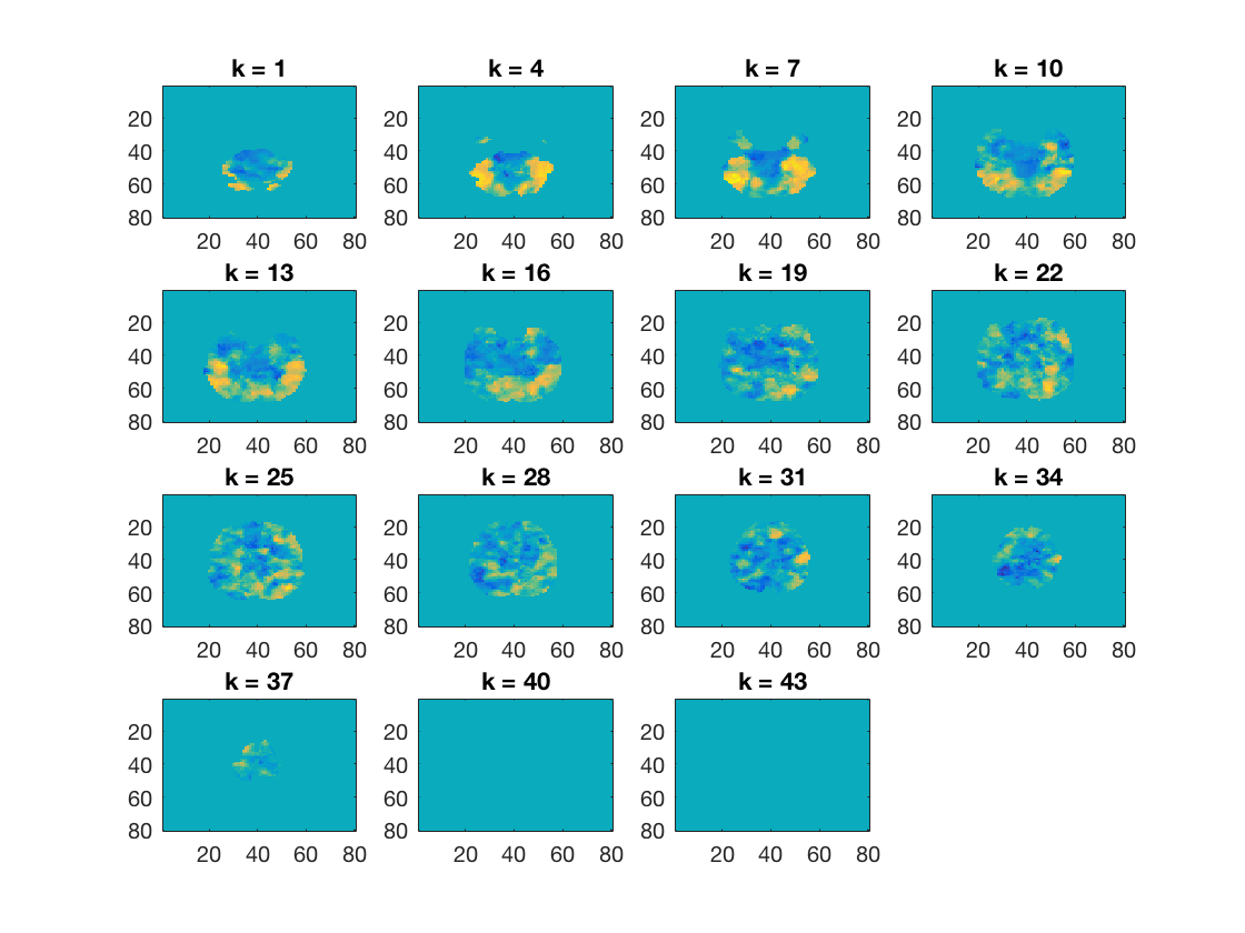
Simple RSM searchlight
nsamples=size(ds.samples,1);
target_dsm=zeros(nsamples);

% define 'simple' target structure where primates (monkey, lemur),
% birds (mallard, warbler) and insects (ladybug, lunamoth) are the same
% (distance=0), all other pairs are equally dissimilar (distance=1).
% Given the ds.sa.targets assignment, pairs (1,2), (3,4) and (5,6) have
% distance 0, all others distance 1.
animal_class=ds.sa.animal_class;
for row=1:nsamples
    for col=1:nsamples
        same_animal_class=animal_class(row)==animal_class(col);

        if same_animal_class
            target_dsm(row,col)=0;
        else
            target_dsm(row,col)=1;
        end
    end
end

fprintf('Using the following target dsm\n');
disp(target_dsm);
imagesc(target_dsm)
set(gca,'XTick',1:nsamples,'XTickLabel',ds.sa.labels,...
        'YTick',1:nsamples,'YTickLabel',ds.sa.labels)

% set measure
measure=@cosmo_target_dsm_corr_measure;
measure_args=struct();
measure_args.target_dsm=target_dsm;

% print measure and arguments
fprintf('Searchlight measure:\n');
cosmo_disp(measure);
fprintf('Searchlight measure arguments:\n');
cosmo_disp(measure_args);

% run searchlight
ds_rsm_binary=cosmo_searchlight(ds,nbrhood,measure,measure_args);

% Note: when these results are used for group analysis across multiple
% participants, it may be good to Fisher-transform the correlation values,
% so that they are more normally distributed. This can be done by:
%
% ds_rsm_binary.samples=atanh(ds_rsm_binary.samples);


% show results
cosmo_plot_slices(ds_rsm_binary);

% store results
output_fn=fullfile(output_path,'rsm_binary.nii');
cosmo_map2fmri(ds_rsm_binary,output_fn);
Using the following target dsm
     0     0     1     1     1     1
     0     0     1     1     1     1
     1     1     0     0     1     1
     1     1     0     0     1     1
     1     1     1     1     0     0
     1     1     1     1     0     0

Searchlight measure:
@cosmo_t ... measure
Searchlight measure arguments:
.target_dsm
  [ 0         0         1         1         1         1
    0         0         1         1         1         1
    1         1         0         0         1         1
    1         1         0         0         1         1
    1         1         1         1         0         0
    1         1         1         1         0         0 ]
+00:00:27 [####################] -00:00:00

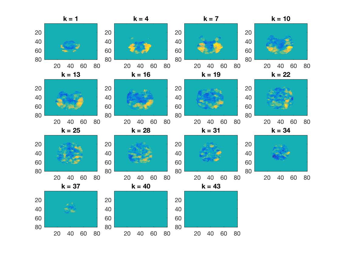
Using another RSM
% This example is very similar to the previous example.
% - This example uses a different target representational similarity
%   matrix. The code below allows for identifying regions that show a
%   linear dissimilarity across animal class, with primates of distance 1
%   from birdsand distance 2 from insects, and insects distance 1 from
%   birds. Graphically:
%
%            +------------------+------------------+
%        primates             birds             insects
%     {monkey,lemur}     {mallard,warbler}   {ladybug,lunamoth}
%
% - It uses a Spearman rather than Pearson correlation measure to match
%   the neural similarity to the target similarity measure

animal_class=ds.sa.animal_class;

% compute absolute difference between each pair of samples
target_dsm=abs(bsxfun(@minus,animal_class,animal_class'));

fprintf('Using the following target dsm\n');
disp(target_dsm);
imagesc(target_dsm)
set(gca,'XTick',1:nsamples,'XTickLabel',ds.sa.labels,...
        'YTick',1:nsamples,'YTickLabel',ds.sa.labels)

% set measure
measure=@cosmo_target_dsm_corr_measure;
measure_args=struct();
measure_args.target_dsm=target_dsm;

% 'Spearman' requires  matlab with stats toolbox; if not present use
% 'Pearson'
if cosmo_check_external('@stats',false)
    measure_args.type='Spearman';
else
    measure_args.type='Pearson';
    fprintf('Matlab stats toolbox not present, using %s correlation\n',...
                measure_args.type)
end

% run searchlight
ds_rsm_linear=cosmo_searchlight(ds,nbrhood,measure,measure_args);

% Note: when these results are used for group analysis across multiple
% participants, it may be good to Fisher-transform the correlation values,
% so that they are more normally distributed. This can be done by:
%
% ds_rsm_linear.samples=atanh(ds_rsm_linear.samples);

% show results
cosmo_plot_slices(ds_rsm_linear);

% store results
output_fn=fullfile(output_path,'rsm_linear.nii');
cosmo_map2fmri(ds_rsm_linear,output_fn);
Using the following target dsm
     0     0     1     1     2     2
     0     0     1     1     2     2
     1     1     0     0     1     1
     1     1     0     0     1     1
     2     2     1     1     0     0
     2     2     1     1     0     0

+00:00:46 [####################] -00:00:00
Using a behavioural RSM
This example is very similar to the one above, but now the target similarity structure is based on behavioural similarity ratings
% load behavioural similarity matrix from disc
behav_model_fn=fullfile(ak6_study_path,'models','behav_sim.mat');
behav_model=importdata(behav_model_fn);

target_dsm=behav_model;

fprintf('Using the following target dsm\n');
disp(target_dsm);
imagesc(target_dsm)
set(gca,'XTick',1:nsamples,'XTickLabel',ds.sa.labels,...
        'YTick',1:nsamples,'YTickLabel',ds.sa.labels)

% set measure
measure=@cosmo_target_dsm_corr_measure;
measure_args=struct();
measure_args.target_dsm=target_dsm;

% run searchlight
ds_rsm_behav=cosmo_searchlight(ds,nbrhood,measure,measure_args);

% Note: when these results are used for group analysis across multiple
% participants, it may be good to Fisher-transform the correlation values,
% so that they are more normally distributed. This can be done by:
%
% ds_rsm_behav.samples=atanh(ds_rsm_behav.samples);

% show results
cosmo_plot_slices(ds_rsm_behav);

% store results
output_fn=fullfile(output_path,'rsm_behav.nii');
cosmo_map2fmri(ds_rsm_behav,output_fn);

% Show citation information
cosmo_check_external('-cite');
Using the following target dsm
         0    0.1015    1.0520    1.0976    1.6778    1.7459
    0.1015         0    1.0420    1.0512    1.7010    1.7570
    1.0520    1.0420         0    0.3924    1.5359    1.4550
    1.0976    1.0512    0.3924         0    1.4730    1.3987
    1.6778    1.7010    1.5359    1.4730         0    0.1603
    1.7459    1.7570    1.4550    1.3987    0.1603         0

+00:00:26 [####################] -00:00:00
If you use CoSMoMVPA and/or some other toolboxes for a publication, please cite:

J. Shen. NIFTI toolbox. available online from http://www.mathworks.com/matlabcentral/fileexchange/8797-tools-for-nifti-and-analyze-image

N. N. Oosterhof, A. C. Connolly, J. V. Haxby (2016). CoSMoMVPA: multi-modal multivariate pattern analysis of neuroimaging data in Matlab / GNU Octave. Frontiers in Neuroinformatics, doi:10.3389/fninf.2016.00027.. CoSMoMVPA toolbox available online from http://cosmomvpa.org

The Mathworks, Natick, MA, United States. Matlab 9.1.0.441655 (R2016b) (September 7, 2016). available online from http://www.mathworks.com